R Tutorials | Principal Component Analysis (PCA) with R | #rstats
https://global-fintech.blogspot.com/2015/12/pca-r-factominer.html
#rstats
What is Principal Component Analysis (PCA)?
Principal component analysis (PCA) is a technique in statistics used to emphasise the variation and produce strong patterns in a dataset and it is often used to make data easy to explore and visualise. In a nutshell, the PCA helps you to find the principal components of data which represent the underlying structure of the latter. The principal components, in simple words, can be seen as directions or eigenvectors having their eigenvalues where the data is most spread out. However, the amount of eigenvectors/-values is much higher than that of of the principal components. It is equal to the number of dimensions in the dataset. One of the main objectives of the PCA is to reduce the number of dimensions.There are different approaches to conduct a PCA. In this series of our R tutorials, we shall use an example of how the PCA done in R using the library FactoMineR. The corresponding files with examples can be found here. The reader should understand the basics of R.
 |
| Using R for PCA with FactoMineR |
1. Analysing the Dataset in R
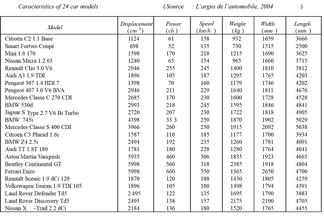
In our example, we shall use a dataset containing the characteristics of 24 car models. The variable Model is qualitative and the further 6 variables (Displacement, Power etc.) are quantitative and continuous.
For the illustration in this part of our R tutorials we use the csv-file "auto2004.csv" (please follow the link to download it). It should be added and attached to the memory of R:
2. Installing FactoMineR
As mentioned before, in this part of our R tutorials we use FactoMineR to conduct a PCA. FactoMineR is an R library created for the purposes of Data Analysis. Among its many methods, FactoMineR can perform the Principal Component Analysis and Cluster Analysis. In order to work with it in R, you need to install it by entering library (FactoMineR) in your R GUI. Make sure that you have installed the dependent libraries such as lme4.
Here is the code in R for installing FactoMineR:
library(FactoMineR).
We conduct a PCA of the quantitative values (rows 3 - 8) of the dataset 'auto' which we have attached previously (see above). We choose to scale the data and select the 6 dimensions in the sample. In this case we do not need to plot the graph.
The next step is to analyse the eigenvalue:
We choose the number of components provided that the total eigenvalue does not descend below 5% and the cumulative percentage is no less than 80%. Therefore, we select two factors.
Next, we build a barplot of the eigenvalues:
 |
| FactoMineR is an R library for Data Analysis |
Here is the code in R for installing FactoMineR:
library(FactoMineR).
3. PCA in R
Once you have installed the FactoMineR, you can conduct the PCA of the dataset. The first action would be to assign the results of the PCA to the value res.pca:
The next step is to analyse the eigenvalue:
 |
| The function res.pca$eig gives the eigenvalues of the principal components and the percentage of the explained variance. |
Next, we build a barplot of the eigenvalues:
barplot(res.pca$eig[,1]) |
| The barplot helps us to determine the number of principal components graphically |
Having done that, we receive two graphs from R, namely:
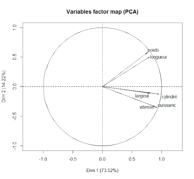
- Variables Factor Map
 |
| The Variable Factor Map shows the correlation of the significant variables and gives an understanding of how individual observations will be scattered along the Individual Factor Map |
- Individuals Factor Map
 |
| The Individual Factor Map explaining 87.7% of the total variance shows the position of the observations according to the factors |
The individuals factor map is interpreted based on the variables factor map.
Next, the function res.pca$ind$coord gives the coordinates of the subjects with respect to the factors. The function res.pca$var$cor gives the correlations between the variables and the factors. To interpret the principal components we use the function dimdesc:
dimdesc(res.pca, axes=c(1,2))
Next, the function res.pca$ind$coord gives the coordinates of the subjects with respect to the factors. The function res.pca$var$cor gives the correlations between the variables and the factors. To interpret the principal components we use the function dimdesc:
dimdesc(res.pca, axes=c(1,2))
The complete illustration of all our R tutorials with comments and the dataset you can find in GitHub.
